Super Bowl Costs
A near national holiday, the Super Bowl is an annual tradition. The NFL championship game is one of the most watched American telecast every year. Because of this, the costs surrounding a Super Bowl are quite large. Today we will take a look at the cost to air a thirty second commercial during the broadcast as well as the ticket price to actually attend the game. For what its worth, this type of analysis is not the first: countless others have taken a look at some or all of this before. However, I will do it again myself and since this is a blog with an analytics bent, I will go beyond the typical viz people have done for this in the past.
The data
I scraped the conveniently named website SuperBowl-Ads.com to obtain the average cost of airing a thirty second commercial. This data, provided by Nielsen Media Research, goes back all the way to Super Bowl I in 1967 when it was in fact simulcast by CBS and NBC. These two networks charged two different prices, so I averaged the two. All other games only had one broadcast network.
To determine ticket prices for the Super Bowl, I decided to use the average (known) face value. This is important for a few reasons. First, the secondary market prices are not known for the older Super Bowls. Second, even if we did, there would have to be a judgement on when to calculate an average since ticket prices fluctuate over time. Thus, it is much safer, and easier, to use the face value of a ticket. To this end, I scraped the table listed at a Syracuse.com article. This table has the last three Super Bowls missing. I was able to find sources for Super Bowls XLVIII and 50 (from Fortune and CNNMoney, respectively) but could not for Super Bowl LI. For this reason, I omitted the cost of a thirty second commercial for Super Bowl LI. It also means a nice even 50 data points for each. Pretty.
Finally, I used the Consumer Price Index from the US Department of Labor to calculate the inflation rates over the years. This is used, of course, to compare historical amounts to present day amounts.
Looking over the years
Plotting the data, we can first take a look at the cost of a (thirty second) commercial. This can be found below. Notice first that the x-axis is the year in which the Super Bowl took place, which is always the year after the football season has already started. So 2016 refers to Super Bowl 50 which took place at the end of the 2015/16 NFL season. Secondly, the inflation adjusted cost of a commercial is in green while the unadjusted average cost is in blue. The green makes it a little easier to compare since the dollar amount can be compared directly. Lastly, note that the left and right panels are both the same. The only difference is the y-scale: the left has a linear axis while the right has a logarithmic axis.
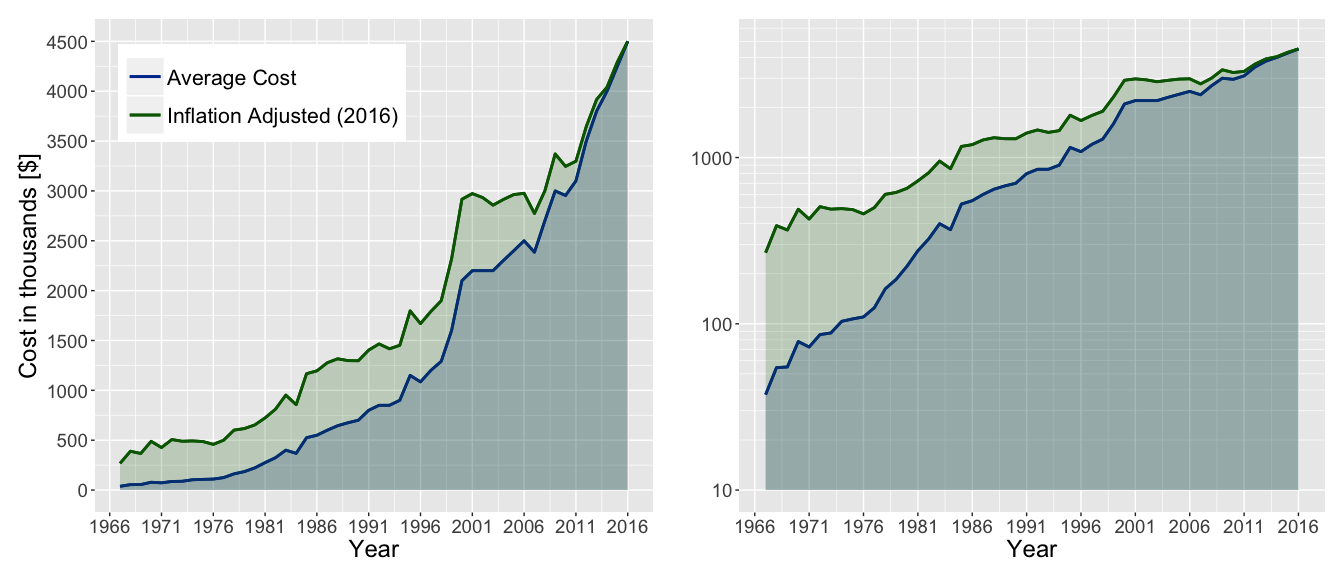
Even adjusting for inflation, the cost to air a commercial continues to go up. The largest spike occurs in the late 1990s/early 2000s i.e. the dot-com boom. The last several years has also seen consistent year to year growth, with the cost increasing at least 5% every year.
We can make the same plot(s) for the average ticket price for every Super Bowl. Recall this is only the face value of tickets. Here we can see that ticket prices were relatively stable in the first two decades or so: the inflation adjusted price hovered around $100 during that time. From the late 1980s onwards though, there has been sustained increases in the price. While there were a few Super Bowls where the ticket price decreased from the previous year, the general trend is clearly pointing upwards. The last few years especially has seen a price hike.

Fitting the growth
The phrase “exponential increase” is often used to describe the costs of airing commercials and purchasing tickets. I wanted to test that. Can an exponential function actually describe either dataset?
For the fitting to follow, I used two separate functional forms:
- Exponential : y = AeBx + C
- Polynomial : y = Ax3 + Bx2 + Cx + D
First, we fit the cost of a commercial. The results of the fitting are shown below. The top panel shows both fits in solid lines while the actual costs are in black points. The bottom panel shows the residuals for each fit. Note the color scheme is the same for both panels.
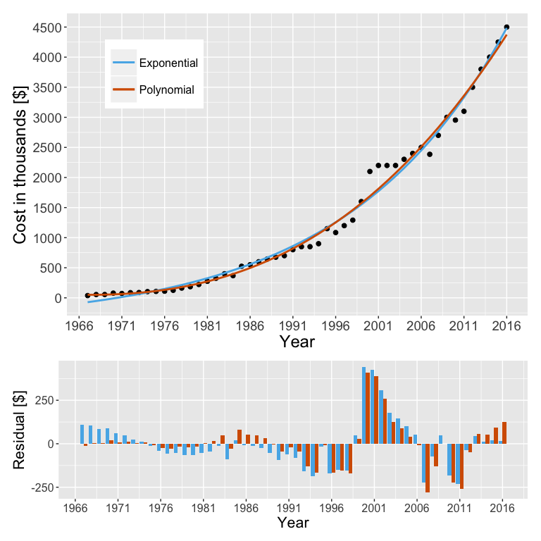
From the eye test you can see both fits actually do a pretty good job. In the first few years, the exponential fit actually is negative and thus has much larger residuals than the polynomial fit in that time period. However, the exponential fit performs better in the last few years as the cost is increasing rather quickly here. In the middle intervening period, it does seem like the polynomial fit performs slightly better. We can use a few statistical tests to compare the two models: the Bayesian information criterion (BIC) and the corrected Akaike information criterion (AICc). For both tests, a smaller value is better. A table summarizing this is given below.
| BIC | AICc | |
|---|---|---|
| Exponential | 648.5 | 641.7 |
| Polynomial | 645.9 | 637.7 |
Both tests yield similar values for each fit. The polynomial fit is lower though suggesting it is the (slightly) better fit. This seemingly confirms what we saw from the eye test. So is it appropriate to say the cost of commercials goes up exponentially? I would say so. While a cubic seems to be more accurate, both can model the cost well.
We will of course repeat this process for the ticket prices. The same functional forms are used here as well. The results of the fit are given below in the same format.
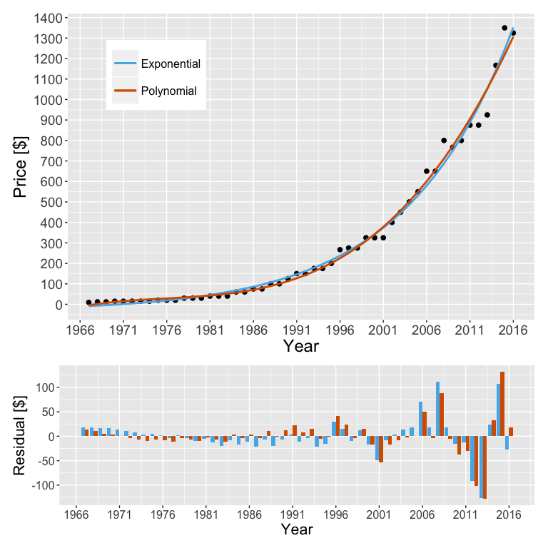
Both fits perform similarly well again in this case. From the eye test it is not immediately obvious which one might be better this time around though. We can repeat the calculations for the BIC and AICc to determine which one might be the superior fit.
| BIC | AICc | |
|---|---|---|
| Exponential | 515.9 | 509.1 |
| Polynomial | 521.2 | 513.0 |
As last time, there is not too much of a difference between the two models. However, both statistical tests do give the edge to the exponential fit. So in the case of the price of a ticket, I would say it is probably appropriate to say it increases exponentially. Though again like last time, the other (i.e. cubic) model can also work.
Predicting the future
Given we seem to have a good working model (or two) for both datasets, we can make some predictions! We can simply use both models on upcoming years and see what the possibilities might be. First up, we take a look at the cost of airing a commercial. The figure below shows a similar plot as the fit result but with a modified x-axis range. Here, the year starts at 1996 and ends at 2026. Thus, I make a prediction for the next ten years. Of course, these are predictions for years into the future so we will not be able to test the model for a number of years. The shaded region for each model represents the error on the prediction (calculated using the delta method).
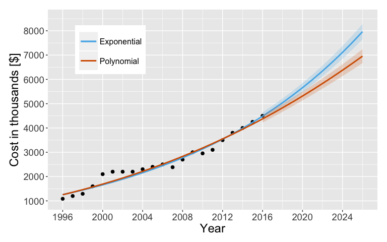
Using this plot, we can read off some numbers. From the plot then, it will take about six (ten) years for the cost of airing a commercial to reach $6 (7) million. It is also entirely possible that within a decade, the cost could be as much as $8 million!
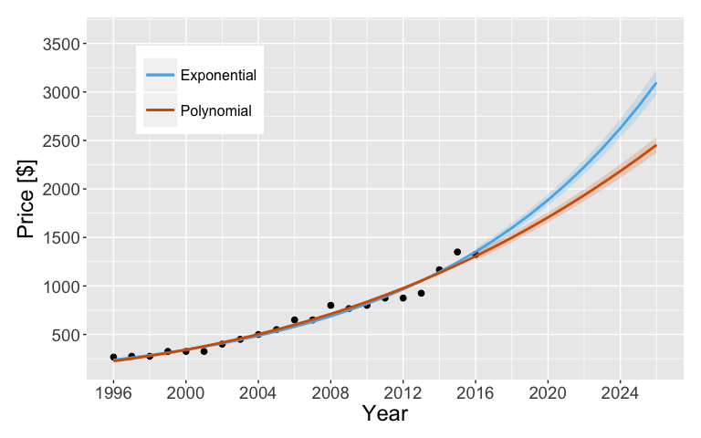
Now let us check out the same plot for the ticket prices. The average face value of a ticket should cost $1,500 within two years, at most. Within about six (ten) years, the price will have jumped to $2,000 (2,500). An average face value of $3,000 is reasonable within a decade as well. Yikes. For someone who does wish to attend a Super Bowl once, I do hope the price these predictions are over-estimated.
Parting thoughts
While there have been many analyses looking at the cost to air a thirty second commercial and the average face value of a ticket at the Super Bowl, I did my own version. Since the common sentiment is that these values seem to go up exponentially, I tested this hypothesis. It turns out to be fairly accurate and given the fits that I did, I made some predictions about future Super Bowls. I can start checking the validity of my fits in a year or two, so I do look forward to the next few Super Bowls.