(Machine) Learning from the Titanic
This is my first attempt at looking at the RMS Titanic dataset on kaggle. This has been described several times, with many tutorials. This is a list of passengers from the Titanic and the purpose of this long-running kaggle competition is to predict which passengers survived the shipwreck. To start we can load in the data and take a peek at what is inside. I am going to take a look at it using R.
train.col <- c('integer',    # PassengerId
                'factor',    # Survived
                'factor',    # Pclass
                'character', # Name
                'factor',    # Sex
                'numeric',   # Age
                'integer',   # SibSp
                'integer',   # Parch
                'character', # Ticket
                'numeric',   # Fare
                'character', # Cabin
                'factor'     # Embarked
               )
test.col <- train.col[-2]    # no Survived column in test.csv

train <- read.csv("train.csv", colClasses = train.col, na.strings = c(""))
test  <- read.csv( "test.csv", colClasses =  test.col, na.strings = c(""))
all <- merge(train, test, all = TRUE)
str(all)
## 'data.frame':    1309 obs. of  12 variables:
##  $ PassengerId: int  1 2 3 4 5 6 7 8 9 10 ...
##  $ Pclass     : Factor w/ 3 levels "1","2","3": 3 1 3 1 3 3 1 3 3 2 ...
##  $ Name       : chr  "Braund, Mr. Owen Harris" "Cumings, Mrs. John Bradley (Florence Briggs Thayer)" "Heikkinen, Miss. Laina" "Futrelle, Mrs. Jacques Heath (Lily May Peel)" ...
##  $ Sex        : Factor w/ 2 levels "female","male": 2 1 1 1 2 2 2 2 1 1 ...
##  $ Age        : num  22 38 26 35 35 NA 54 2 27 14 ...
##  $ SibSp      : int  1 1 0 1 0 0 0 3 0 1 ...
##  $ Parch      : int  0 0 0 0 0 0 0 1 2 0 ...
##  $ Ticket     : chr  "A/5 21171" "PC 17599" "STON/O2. 3101282" "113803" ...
##  $ Fare       : num  7.25 71.28 7.92 53.1 8.05 ...
##  $ Cabin      : chr  NA "C85" NA "C123" ...
##  $ Embarked   : Factor w/ 3 levels "C","Q","S": 3 1 3 3 3 2 3 3 3 1 ...
##  $ Survived   : Factor w/ 2 levels "0","1": 1 2 2 2 1 1 1 1 2 2 ...
summary(all)
##   PassengerId   Pclass      Name               Sex           Age
##  Min.   :   1   1:323   Length:1309        female:466   Min.   : 0.17
##  1st Qu.: 328   2:277   Class :character   male  :843   1st Qu.:21.00
##  Median : 655   3:709   Mode  :character                Median :28.00
##  Mean   : 655                                           Mean   :29.88
##  3rd Qu.: 982                                           3rd Qu.:39.00
##  Max.   :1309                                           Max.   :80.00
##                                                         NA's   :263
##      SibSp            Parch          Ticket               Fare
##  Min.   :0.0000   Min.   :0.000   Length:1309        Min.   :  0.000
##  1st Qu.:0.0000   1st Qu.:0.000   Class :character   1st Qu.:  7.896
##  Median :0.0000   Median :0.000   Mode  :character   Median : 14.454
##  Mean   :0.4989   Mean   :0.385                      Mean   : 33.295
##  3rd Qu.:1.0000   3rd Qu.:0.000                      3rd Qu.: 31.275
##  Max.   :8.0000   Max.   :9.000                      Max.   :512.329
##                                                      NA's   :1
##     Cabin           Embarked   Survived
##  Length:1309        C   :270   0   :549
##  Class :character   Q   :123   1   :342
##  Mode  :character   S   :914   NA's:418
##                     NA's:  2
##
##
##
We merge both the training and test set so that we can take a look at everything all at once. The first thing to take a look at is to see what is actually present in the dataset. We can do that below in graphical and tabular forms.
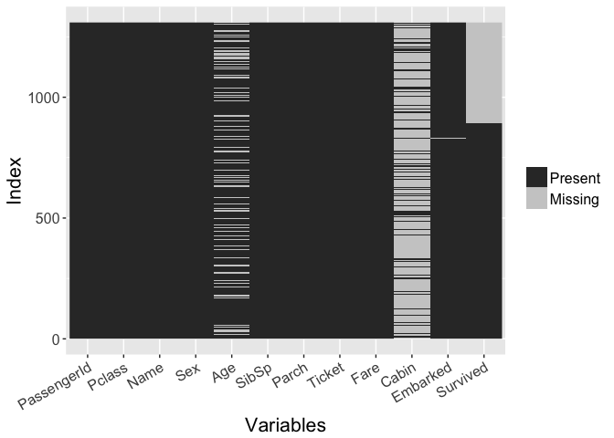
sapply(all, function(x) sum(is.na(x)))
## PassengerId      Pclass        Name         Sex         Age       SibSp
##           0           0           0           0         263           0
##       Parch      Ticket        Fare       Cabin    Embarked    Survived
##           0           0           1        1014           2         418
Interestingly, the dataset is mostly complete. It seems to be missing some 20% of the Age column and some 90% of the Cabin column. Of course there is a huge chunk of survived missing, but that is the actual test data. Now we can see that we might be able to better estimate the missing Age data given the information we have from all the passengers. The Cabin data is still very sparse, so it will be tough to use this variable. But part of this type of estimate (imputation) will require some feature engineering. That is we can try to learn some things about existing info/columns to try to extract some additional knowledge.
Feature engineering
Titles
So let’s take a look again at the data. Recall the point of this exercise is to predict the passengers who survived in the test dataset.
head(all)
##   PassengerId Pclass                                                Name
## 1           1      3                             Braund, Mr. Owen Harris
## 2           2      1 Cumings, Mrs. John Bradley (Florence Briggs Thayer)
## 3           3      3                              Heikkinen, Miss. Laina
## 4           4      1        Futrelle, Mrs. Jacques Heath (Lily May Peel)
## 5           5      3                            Allen, Mr. William Henry
## 6           6      3                                    Moran, Mr. James
##      Sex Age SibSp Parch           Ticket    Fare Cabin Embarked Survived
## 1   male  22     1     0        A/5 21171  7.2500  <NA>        S        0
## 2 female  38     1     0         PC 17599 71.2833   C85        C        1
## 3 female  26     0     0 STON/O2. 3101282  7.9250  <NA>        S        1
## 4 female  35     1     0           113803 53.1000  C123        S        1
## 5   male  35     0     0           373450  8.0500  <NA>        S        0
## 6   male  NA     0     0           330877  8.4583  <NA>        Q        0
We can notice the Name field actually includes the title of a passenger. Considering the time period, these titles can help provide some info. So let’s try to extract that info using some reg-ex.
all$Title <- gsub("^.*, (.*?)\\..*$", "\\1", all$Name)
table(all$Sex, all$Title)
##
##          Capt Col Don Dona  Dr Jonkheer Lady Major Master Miss Mlle Mme
##   female    0   0   0    1   1        0    1     0      0  260    2   1
##   male      1   4   1    0   7        1    0     2     61    0    0   0
##
##           Mr Mrs  Ms Rev Sir the Countess
##   female   0 197   2   0   0            1
##   male   757   0   0   8   1            0
I used the table function to show how many Titles there are (17) and to which gender each belongs. The vast majority of passengers either were addressed by Mr. or Mrs./Miss. There are a few Titles which are only used a few times. Let’s take a closer look at those:
- Captain - Military rank (one below Major)
- Don - Spanish, Portuguese, and Italian male honorific
- Dona - Female version of Don
- Jonkheer - Dutch male honorific
- Lady - English female honorific
- Major - Military rank (one above Captain)
- Mademoiselle (Mlle) - French form of (polite) address for unmarried females, similar to the English ‘Miss’
- Madame (Mme) - French form of (polite) address for females, similar to the English ‘Mrs.’
- Ms - English form of address for females (regardless of marital status)
- Sir - English male honorific
- Countess - English title of nobility for females
It becomes obvious that some of these Titles can be combined into one. We can again use gsub to accomplish this task.
all$Title <- gsub("Dona|Lady|the Countess", "Lady", all$Title)
all$Title <- gsub("Mlle", "Miss", all$Title)
all$Title <- gsub("Mme", "Mrs", all$Title)
all$Title <- gsub("Don|Jonkheer|Sir", "Sir", all$Title)
So, we’re able to reduce the number of Titles to 12. I also want to take a look at the 7 military officers on board the ship.
subset(all, Title == "Capt" | Title == "Major" | Title == "Col")
##      PassengerId Pclass                                Name  Sex Age SibSp
## 450          450      1      Peuchen, Major. Arthur Godfrey male  52     0
## 537          537      1   Butt, Major. Archibald Willingham male  45     0
## 648          648      1 Simonius-Blumer, Col. Oberst Alfons male  56     0
## 695          695      1                     Weir, Col. John male  60     0
## 746          746      1        Crosby, Capt. Edward Gifford male  70     1
## 1023        1023      1           Gracie, Col. Archibald IV male  53     0
## 1094        1094      1              Astor, Col. John Jacob male  47     1
##      Parch    Ticket    Fare   Cabin Embarked Survived Title
## 450      0    113786  30.500    C104        S        1 Major
## 537      0    113050  26.550     B38        S        0 Major
## 648      0     13213  35.500     A26        C        1   Col
## 695      0    113800  26.550    <NA>        S        0   Col
## 746      1 WE/P 5735  71.000     B22        S        0  Capt
## 1023     0    113780  28.500     C51        C     <NA>   Col
## 1094     0  PC 17757 227.525 C62 C64        C     <NA>   Col
We can see they are generally around the same Age, travelling in the top 3 cabins available and paid around the same price for their tickets. I think it is fair to lump them into one Title, so we’ll upgrade some of them to the rank of Colonel.
all$Title <- gsub("Capt|Major|Col", "Col", all$Title)
Since there are only two passengers with the Title ‘Ms,’ I want to try to reclassify those Titles as well.
subset(all, Title == "Ms")
##     PassengerId Pclass                      Name    Sex Age SibSp Parch
## 444         444      2 Reynaldo, Ms. Encarnacion female  28     0     0
## 980         980      3   O'Donoghue, Ms. Bridget female  NA     0     0
##     Ticket  Fare Cabin Embarked Survived Title
## 444 230434 13.00  <NA>        S        1    Ms
## 980 364856  7.75  <NA>        Q     <NA>    Ms
If we take a look at the history of both these passengers at the Encyclopedia Titanica. We can see that Ms. Reynaldo was a widow and Ms. O’Donoghue was never married. So I will change their Titles to Miss.
all$Title <- gsub("Ms", "Miss", all$Title)
all$Title <- as.factor(all$Title) #Make sure its a factor
table(all$Sex, all$Title)
##
##          Col  Dr Lady Master Miss  Mr Mrs Rev Sir
##   female   0   1    3      0  264   0 198   0   0
##   male     7   7    0     61    0 757   0   8   3
str(all)
## 'data.frame':    1309 obs. of  13 variables:
##  $ PassengerId: int  1 2 3 4 5 6 7 8 9 10 ...
##  $ Pclass     : Factor w/ 3 levels "1","2","3": 3 1 3 1 3 3 1 3 3 2 ...
##  $ Name       : chr  "Braund, Mr. Owen Harris" "Cumings, Mrs. John Bradley (Florence Briggs Thayer)" "Heikkinen, Miss. Laina" "Futrelle, Mrs. Jacques Heath (Lily May Peel)" ...
##  $ Sex        : Factor w/ 2 levels "female","male": 2 1 1 1 2 2 2 2 1 1 ...
##  $ Age        : num  22 38 26 35 35 NA 54 2 27 14 ...
##  $ SibSp      : int  1 1 0 1 0 0 0 3 0 1 ...
##  $ Parch      : int  0 0 0 0 0 0 0 1 2 0 ...
##  $ Ticket     : chr  "A/5 21171" "PC 17599" "STON/O2. 3101282" "113803" ...
##  $ Fare       : num  7.25 71.28 7.92 53.1 8.05 ...
##  $ Cabin      : chr  NA "C85" NA "C123" ...
##  $ Embarked   : Factor w/ 3 levels "C","Q","S": 3 1 3 3 3 2 3 3 3 1 ...
##  $ Survived   : Factor w/ 2 levels "0","1": 1 2 2 2 1 1 1 1 2 2 ...
##  $ Title      : Factor w/ 9 levels "Col","Dr","Lady",..: 6 7 5 7 6 6 6 4 7 7 ...
Group Sizes
So I have reduced the number of Titles in half to 9 from the original 18. I think this introduces a lot of extra info we had from the Name column, but in a compact way. Next we can focus on the Ticket column. These are the ticket numbers for each passenger. From previous printouts we know that some of the ticket information includes a character string. We can strip this info and keep just the ticket number itself. However, if we look carefully at the Ticket info, there are four that have the string ‘LINE’ listed.
subset(all, Ticket=="LINE")
##     PassengerId Pclass                            Name  Sex Age SibSp
## 180         180      3             Leonard, Mr. Lionel male  36     0
## 272         272      3    Tornquist, Mr. William Henry male  25     0
## 303         303      3 Johnson, Mr. William Cahoone Jr male  19     0
## 598         598      3             Johnson, Mr. Alfred male  49     0
##     Parch Ticket Fare Cabin Embarked Survived Title
## 180     0   LINE    0  <NA>        S        0    Mr
## 272     0   LINE    0  <NA>        S        1    Mr
## 303     0   LINE    0  <NA>        S        0    Mr
## 598     0   LINE    0  <NA>        S        0    Mr
For whatever reason, these four Tickets are not correctly listed. Further, these four passengers do not seem to be related. So I will insert an arbitrary set of strings to replace the ‘LINE.’
all[subset(all, Ticket=="LINE")$PassengerId, "Ticket"] <- c("99991","99992","99993","99994")
With that done, we can finally get the TicketNo extracted.
all$TicketNo <- gsub("[^0-9]", "", all$Ticket)
head(all)
##   PassengerId Pclass                                                Name
## 1           1      3                             Braund, Mr. Owen Harris
## 2           2      1 Cumings, Mrs. John Bradley (Florence Briggs Thayer)
## 3           3      3                              Heikkinen, Miss. Laina
## 4           4      1        Futrelle, Mrs. Jacques Heath (Lily May Peel)
## 5           5      3                            Allen, Mr. William Henry
## 6           6      3                                    Moran, Mr. James
##      Sex Age SibSp Parch           Ticket    Fare Cabin Embarked Survived
## 1   male  22     1     0        A/5 21171  7.2500  <NA>        S        0
## 2 female  38     1     0         PC 17599 71.2833   C85        C        1
## 3 female  26     0     0 STON/O2. 3101282  7.9250  <NA>        S        1
## 4 female  35     1     0           113803 53.1000  C123        S        1
## 5   male  35     0     0           373450  8.0500  <NA>        S        0
## 6   male  NA     0     0           330877  8.4583  <NA>        Q        0
##   Title TicketNo
## 1    Mr   521171
## 2   Mrs    17599
## 3  Miss 23101282
## 4   Mrs   113803
## 5    Mr   373450
## 6    Mr   330877
This will allow us to see that some people traveled together on the same ticket. We do have two fields SibSp and Parch which give us the the sibling plus spouse and parent plus children counts on board, respectively. We can combine these two to compare to our TicketNo info. The way to do this is to count every passenger travelling on the same ticket first. We can do that by using the ddply method alongside transform to do this counting for us.
all$FamilySize <- all$SibSp + all$Parch
all <- ddply(all, ~ TicketNo, transform, TravelSize = length(TicketNo)-1 )
head(all)
##   PassengerId Pclass
## 1         258      1
## 2         505      1
## 3         760      1
## 4         263      1
## 5         559      1
## 6         586      1
##                                                       Name    Sex Age
## 1                                     Cherry, Miss. Gladys female  30
## 2                                    Maioni, Miss. Roberta female  16
## 3 Rothes, the Countess. of (Lucy Noel Martha Dyer-Edwards) female  33
## 4                                        Taussig, Mr. Emil   male  52
## 5                   Taussig, Mrs. Emil (Tillie Mandelbaum) female  39
## 6                                      Taussig, Miss. Ruth female  18
##   SibSp Parch Ticket  Fare Cabin Embarked Survived Title TicketNo
## 1     0     0 110152 86.50   B77        S        1  Miss   110152
## 2     0     0 110152 86.50   B79        S        1  Miss   110152
## 3     0     0 110152 86.50   B77        S        1  Lady   110152
## 4     1     1 110413 79.65   E67        S        0    Mr   110413
## 5     1     1 110413 79.65   E67        S        1   Mrs   110413
## 6     0     2 110413 79.65   E68        S        1  Miss   110413
##   FamilySize TravelSize
## 1          0          2
## 2          0          2
## 3          0          2
## 4          2          2
## 5          2          2
## 6          2          2
Now, we can plot the TravelSize against the FamilySize to see how they each compare. Because the FamilySize only captures certain familial relations, people travelling on the same ticket could be other relations, friends, or neighbors. This means our calculated TravelSize could capture some additional information missing in FamilySize. Of course, this does not need to be true.
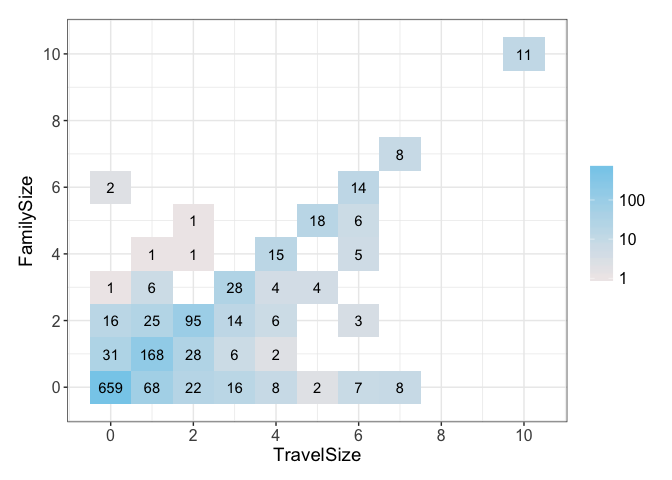
The plot shows there is a correlation between the two. However it also shows that there differences between the two, so it reinforces our hypothesis that the TravelSize might be capturing additional information.
Missing data
We also remember from the start that there are some pieces of data missing, some much bigger than others. Let’s take a look again at what we do not have.
summary(all)
##   PassengerId   Pclass      Name               Sex           Age
##  Min.   :   1   1:323   Length:1309        female:466   Min.   : 0.17
##  1st Qu.: 328   2:277   Class :character   male  :843   1st Qu.:21.00
##  Median : 655   3:709   Mode  :character                Median :28.00
##  Mean   : 655                                           Mean   :29.88
##  3rd Qu.: 982                                           3rd Qu.:39.00
##  Max.   :1309                                           Max.   :80.00
##                                                         NA's   :263
##      SibSp            Parch          Ticket               Fare
##  Min.   :0.0000   Min.   :0.000   Length:1309        Min.   :  0.000
##  1st Qu.:0.0000   1st Qu.:0.000   Class :character   1st Qu.:  7.896
##  Median :0.0000   Median :0.000   Mode  :character   Median : 14.454
##  Mean   :0.4989   Mean   :0.385                      Mean   : 33.295
##  3rd Qu.:1.0000   3rd Qu.:0.000                      3rd Qu.: 31.275
##  Max.   :8.0000   Max.   :9.000                      Max.   :512.329
##                                                      NA's   :1
##     Cabin           Embarked   Survived       Title       TicketNo
##  Length:1309        C   :270   0   :549   Mr     :757   Length:1309
##  Class :character   Q   :123   1   :342   Miss   :264   Class :character
##  Mode  :character   S   :914   NA's:418   Mrs    :198   Mode  :character
##                     NA's:  2              Master : 61
##                                           Dr     :  8
##                                           Rev    :  8
##                                           (Other): 13
##    FamilySize        TravelSize
##  Min.   : 0.0000   Min.   : 0.000
##  1st Qu.: 0.0000   1st Qu.: 0.000
##  Median : 0.0000   Median : 0.000
##  Mean   : 0.8839   Mean   : 1.105
##  3rd Qu.: 1.0000   3rd Qu.: 2.000
##  Max.   :10.0000   Max.   :10.000
##
We are missing Age, Fare, and Embarked info from the NA that shows up. We also know most of the Cabin information is missing. Let’s start with missing Fares.
Fare
As usual, we start with a distribution and some statistics.
##    Min. 1st Qu.  Median    Mean 3rd Qu.    Max.    NA's
##   0.000   7.896  14.450  33.300  31.280 512.300       1
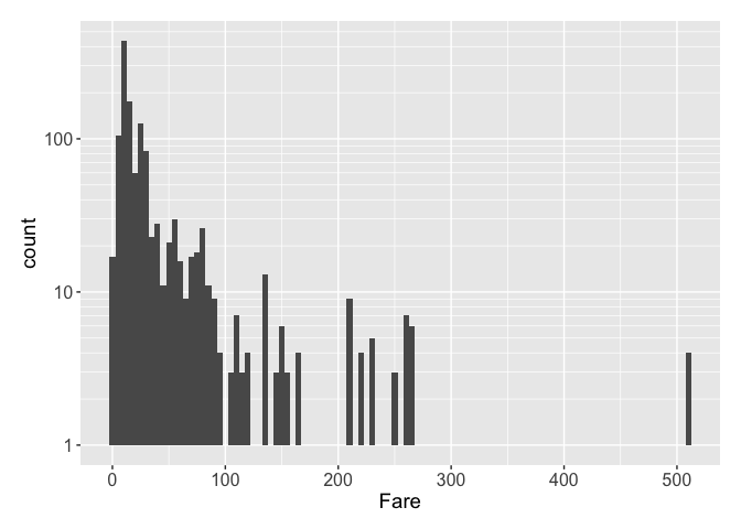
We see an interesting bin: there are a dozen or so Fares with zero (what unit exactly??). Let’s take a look at these passengers; they could be infants.
subset(all, Fare == 0)
##      PassengerId Pclass                                  Name  Sex Age
## 23           807      1                Andrews, Mr. Thomas Jr male  39
## 24          1158      1 Chisholm, Mr. Roderick Robert Crispin male  NA
## 25           634      1         Parr, Mr. William Henry Marsh male  NA
## 27           816      1                      Fry, Mr. Richard male  NA
## 28          1264      1               Ismay, Mr. Joseph Bruce male  49
## 29           264      1                 Harrison, Mr. William male  40
## 334          823      1       Reuchlin, Jonkheer. John George male  38
## 476          278      2           Parkes, Mr. Francis "Frank" male  NA
## 477          414      2        Cunningham, Mr. Alfred Fleming male  NA
## 478          467      2                 Campbell, Mr. William male  NA
## 479          482      2      Frost, Mr. Anthony Wood "Archie" male  NA
## 480          733      2                  Knight, Mr. Robert J male  NA
## 481          675      2            Watson, Mr. Ennis Hastings male  NA
## 1306         180      3                   Leonard, Mr. Lionel male  36
## 1307         272      3          Tornquist, Mr. William Henry male  25
## 1308         303      3       Johnson, Mr. William Cahoone Jr male  19
## 1309         598      3                   Johnson, Mr. Alfred male  49
##      SibSp Parch Ticket Fare       Cabin Embarked Survived Title TicketNo
## 23       0     0 112050    0         A36        S        0    Mr   112050
## 24       0     0 112051    0        <NA>        S     <NA>    Mr   112051
## 25       0     0 112052    0        <NA>        S        0    Mr   112052
## 27       0     0 112058    0        B102        S        0    Mr   112058
## 28       0     0 112058    0 B52 B54 B56        S     <NA>    Mr   112058
## 29       0     0 112059    0         B94        S        0    Mr   112059
## 334      0     0  19972    0        <NA>        S        0   Sir    19972
## 476      0     0 239853    0        <NA>        S        0    Mr   239853
## 477      0     0 239853    0        <NA>        S        0    Mr   239853
## 478      0     0 239853    0        <NA>        S        0    Mr   239853
## 479      0     0 239854    0        <NA>        S        0    Mr   239854
## 480      0     0 239855    0        <NA>        S        0    Mr   239855
## 481      0     0 239856    0        <NA>        S        0    Mr   239856
## 1306     0     0  99991    0        <NA>        S        0    Mr    99991
## 1307     0     0  99992    0        <NA>        S        1    Mr    99992
## 1308     0     0  99993    0        <NA>        S        0    Mr    99993
## 1309     0     0  99994    0        <NA>        S        0    Mr    99994
##      FamilySize TravelSize
## 23            0          0
## 24            0          0
## 25            0          0
## 27            0          1
## 28            0          1
## 29            0          0
## 334           0          0
## 476           0          2
## 477           0          2
## 478           0          2
## 479           0          0
## 480           0          0
## 481           0          0
## 1306          0          0
## 1307          0          0
## 1308          0          0
## 1309          0          0
It does not appear to be the case at all. They are all men who Embarked at Southampton (‘S’) that span all three Pclasses. Let’s redefine these Fares as NA and look at those passengers.
all$Fare[all$Fare == 0] <- NA
all[(which(is.na(all$Fare))),]
##      PassengerId Pclass                                  Name  Sex  Age
## 23           807      1                Andrews, Mr. Thomas Jr male 39.0
## 24          1158      1 Chisholm, Mr. Roderick Robert Crispin male   NA
## 25           634      1         Parr, Mr. William Henry Marsh male   NA
## 27           816      1                      Fry, Mr. Richard male   NA
## 28          1264      1               Ismay, Mr. Joseph Bruce male 49.0
## 29           264      1                 Harrison, Mr. William male 40.0
## 334          823      1       Reuchlin, Jonkheer. John George male 38.0
## 476          278      2           Parkes, Mr. Francis "Frank" male   NA
## 477          414      2        Cunningham, Mr. Alfred Fleming male   NA
## 478          467      2                 Campbell, Mr. William male   NA
## 479          482      2      Frost, Mr. Anthony Wood "Archie" male   NA
## 480          733      2                  Knight, Mr. Robert J male   NA
## 481          675      2            Watson, Mr. Ennis Hastings male   NA
## 1123        1044      3                    Storey, Mr. Thomas male 60.5
## 1306         180      3                   Leonard, Mr. Lionel male 36.0
## 1307         272      3          Tornquist, Mr. William Henry male 25.0
## 1308         303      3       Johnson, Mr. William Cahoone Jr male 19.0
## 1309         598      3                   Johnson, Mr. Alfred male 49.0
##      SibSp Parch Ticket Fare       Cabin Embarked Survived Title TicketNo
## 23       0     0 112050   NA         A36        S        0    Mr   112050
## 24       0     0 112051   NA        <NA>        S     <NA>    Mr   112051
## 25       0     0 112052   NA        <NA>        S        0    Mr   112052
## 27       0     0 112058   NA        B102        S        0    Mr   112058
## 28       0     0 112058   NA B52 B54 B56        S     <NA>    Mr   112058
## 29       0     0 112059   NA         B94        S        0    Mr   112059
## 334      0     0  19972   NA        <NA>        S        0   Sir    19972
## 476      0     0 239853   NA        <NA>        S        0    Mr   239853
## 477      0     0 239853   NA        <NA>        S        0    Mr   239853
## 478      0     0 239853   NA        <NA>        S        0    Mr   239853
## 479      0     0 239854   NA        <NA>        S        0    Mr   239854
## 480      0     0 239855   NA        <NA>        S        0    Mr   239855
## 481      0     0 239856   NA        <NA>        S        0    Mr   239856
## 1123     0     0   3701   NA        <NA>        S     <NA>    Mr     3701
## 1306     0     0  99991   NA        <NA>        S        0    Mr    99991
## 1307     0     0  99992   NA        <NA>        S        1    Mr    99992
## 1308     0     0  99993   NA        <NA>        S        0    Mr    99993
## 1309     0     0  99994   NA        <NA>        S        0    Mr    99994
##      FamilySize TravelSize
## 23            0          0
## 24            0          0
## 25            0          0
## 27            0          1
## 28            0          1
## 29            0          0
## 334           0          0
## 476           0          2
## 477           0          2
## 478           0          2
## 479           0          0
## 480           0          0
## 481           0          0
## 1123          0          0
## 1306          0          0
## 1307          0          0
## 1308          0          0
## 1309          0          0
In order to come up with the Fare imputation, I want to calculate the mean Fare for each Pclass and Title. This is done since all the passengers we care about are all ‘Mr’ (save one). This averaging process is shown below.
df.temp <- subset(all, Embarked == 'S') #Only get Southampton passengers
ddply(df.temp, c("Pclass","Title"), summarize, AveFare = mean(Fare, na.rm = TRUE))
##    Pclass  Title   AveFare
## 1       1    Col  38.65000
## 2       1     Dr  80.47917
## 3       1   Lady  86.50000
## 4       1 Master 117.80277
## 5       1   Miss 127.37830
## 6       1     Mr  55.14049
## 7       1    Mrs  83.35187
## 8       1    Sir       NaN
## 9       2     Dr  12.25000
## 10      2 Master  26.42500
## 11      2   Miss  22.59091
## 12      2     Mr  20.69073
## 13      2    Mrs  23.41122
## 14      2    Rev  19.50357
## 15      3 Master  27.78151
## 16      3   Miss  17.50096
## 17      3     Mr  11.88229
## 18      3    Mrs  19.13560
Now, we can assign those values to those passengers.
df.temp <- ddply(df.temp, c("Pclass","Title"), transform, AveFare = mean(Fare, na.rm = TRUE)) #compute
all[(which(is.na(all$Fare))), "Fare"] <- df.temp[(which(is.na(df.temp$Fare))), "AveFare"] #assign
There is still one passenger who does not have a Fare, and that was the only average Fare we could not compute. Instead, we will treat that passenger as a ‘Mr’ for the purposes of the cost of his ticket. In that case then, we simply assign that value we calculated from before (55).
all[all$PassengerId == 823, "Fare"] <- 55
That takes care of all the Fare data. Next we turn to the Embarked data.
Embarkment
all[(which(is.na(all$Embarked))),]
##    PassengerId Pclass                                      Name    Sex Age
## 59          62      1                       Icard, Miss. Amelie female  38
## 60         830      1 Stone, Mrs. George Nelson (Martha Evelyn) female  62
##    SibSp Parch Ticket Fare Cabin Embarked Survived Title TicketNo
## 59     0     0 113572   80   B28     <NA>        1  Miss   113572
## 60     0     0 113572   80   B28     <NA>        1   Mrs   113572
##    FamilySize TravelSize
## 59          0          1
## 60          0          1
These two passengers, who were travelling on the same ticket and stayed in the same cabin, do not have any Embarkment information. We also know they both paid 80 for each ticket. We can take a look at the usual Fare paid by females for the three ports. This way we can compare the Fares to guess which port is the likeliest.
df.temp <- subset(all, Pclass == 1)
ddply(df.temp, c("Sex","Embarked"), summarize,
      AveFare = mean(Fare, na.rm=TRUE), MedFare = median(Fare, na.rm=TRUE), NumPas = length(Pclass))
##      Sex Embarked   AveFare  MedFare NumPas
## 1 female        C 118.89595 83.15830     71
## 2 female        Q  90.00000 90.00000      2
## 3 female        S 101.06914 78.85000     69
## 4 female     <NA>  80.00000 80.00000      2
## 5   male        C  94.62256 62.66875     70
## 6   male        Q  90.00000 90.00000      1
## 7   male        S  57.24338 44.00000    108
Doing this we see that Southampton is the most likely Embarkment point, since both median and mean are closest to 80. So let’s set this info before continuing.
all[(which(is.na(all$Embarked))), "Embarked"] <- "S"
Age
Now, we can finally tackle the Age data. Unlike the previous columns with missing data, this data is only about 80% complete: some 260 passengers do not have any Age data. So in order to estimate these ages, we will have to go a little deeper into the data. But first, let’s take a cursory look at the data.
##    Min. 1st Qu.  Median    Mean 3rd Qu.    Max.    NA's
##    0.17   21.00   28.00   29.88   39.00   80.00     263
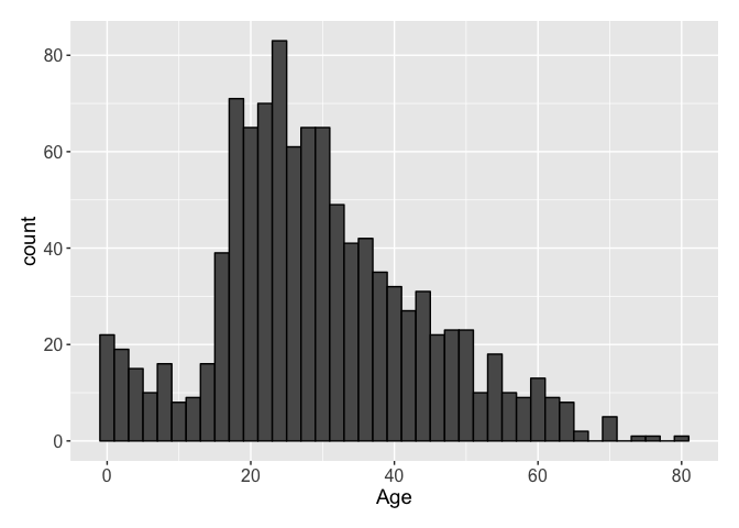
There are no surprises we can see in the Age distribution, with a peak in the number of 20 year-olds. There are a multitude of ways to come up with a way to estimate the missing data. The easiest way is likely fitting a linear model. While I did go through the motions to do that, I wanted something a little more sophisticated. I arbitrarily chose a gradient boosted model to fit the Age. To do this, I used the R packages gbm and caret for the training and fitting. The gradient boosting does require some tuning and I tried a few different options. The model I will show is the one that performed best. Let’s take a look at it.
gbmControl <- trainControl(method='repeatedcv', number = 10, repeats = 10, verboseIter = FALSE,
                           returnResamp = 'all',
                           summaryFunction=defaultSummary)
gbmGrid <-  expand.grid(interaction.depth = c(2, 3),
                    n.trees = (1:20)*20,
                    shrinkage = 0.1, # or something like seq(.001, .1, .01)
                    n.minobsinnode = 10) # or something like c(5, 10, 15, 20)
age.model <- train(Age ~ Pclass + Sex + Fare + Embarked + Title + SibSp + Parch + TravelSize,
                  data = all[!is.na(all$Age), ],
                  method = 'gbm',
                  trControl = gbmControl,
                  tuneGrid = gbmGrid,
                  verbose = FALSE)
This sets up a trained model of Age using all the Age data we have. The fit does a 10-fold CV repeated 10 times. Also notice I did not include the FamilySize variable I added. Instead, it seems to perform slightly worse than the two variables it replaces.
With a model in hand we can take a look at some of its characteristics. First we can use the plot method to see how the model changed with the varying tuning parameters.
plot(age.model)
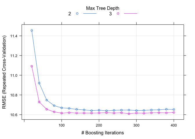
The fit wants to minimize the Root Mean Square Error (RMSE) and we can see that it becomes minimized relatively quickly. The model can also tell us what factors were most important. The very handy varImp function allows us to visualize this easily.
plot(varImp(age.model))
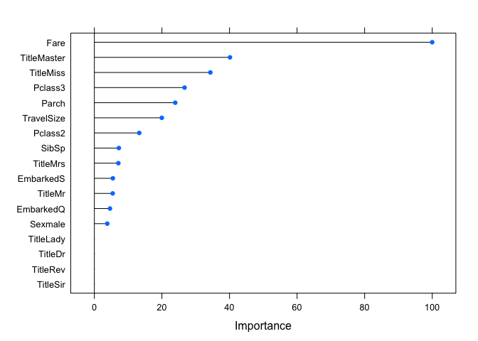
It seems some of the Titles are important to estimating the Age, so it is good we did extract that information earlier. This type of plot helps with understanding the relationships between the factors and the variable we want to predict. Knowing the model a little better, we can predict the missing Ages. Another check we can perform is make sure the predicted value distribution is not too different from the actual values we have. Let’s take a look. The two plots below show both the Age density (top) and histogram (bottom) for the actual (dark gray) and predicted (red) Age values.
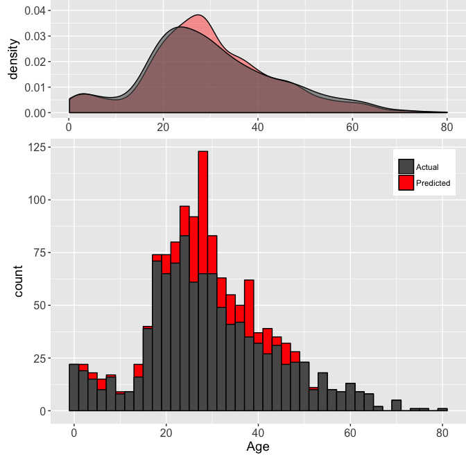
Taking a look at this we can see the model does not seem to make any abnormal predictions. Any peculiar outputs from a model could be a red flag that it is not behaving as desired, so it is important to make these types of sanity checks. A further check of the model is to graph the residuals of the fit. This is done to ensure there does not seem to be any bias from the fit.
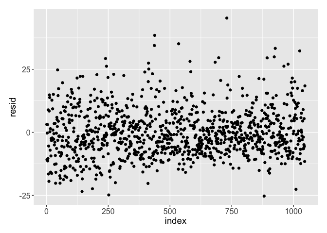
The residuals look to be distributed as expected: it is roughly rectangular with a concentration along zero. We seem to have a good model and estimate for the Age. So let’s fill the NA values with our predictions.
all$Age[is.na(all$Age)] <- predict(age.model, all[is.na(all$Age),])
That takes care of all the missing data, except the Cabin values. Unfortunately it is over three-quarters missing, so any imputation will be very difficult. So I elected to not attempt to estimate this value.
Modeling survival
With the data ready for modeling, let’s split the data frame up again. Recall, we had combined both the training and test data at the beginning of this exercise. Also note that in order to help R with the modeling, we will rename the two levels of the survived variable.
all$Survived <- revalue(all$Survived, c("1" = "Survived", "0" = "Perished"))
train.all <- all[!is.na(all$Survived), ]
 test.all <- all[ is.na(all$Survived), ]
Because I intend to use a few different methods to model whether a passenger survived or not, I will further split the train data. This is done to keep a validation set to compare the performance of the various models we will develop. We will use the createDataPartition method to accomplish this. An 80/20 split of the data will be made.
set.seed(8020)
train.rows <- createDataPartition(train.all$Survived, p = 0.8, list = FALSE)
train.fit <- train.all[ train.rows, ]
 test.fit <- train.all[-train.rows, ]
With a training set ready, now we can start the fitting process. We can start at the simplest fit first: a linear model. We will use a common trainControl method for use in the train method. This control function will perform a 10-fold CV repeated 10 times, as before.
fitControl <- trainControl(method = "repeatedcv", repeats = 10, number = 10,
                           summaryFunction = twoClassSummary,
                           classProbs = TRUE)
Linear models
We will use the glm model. Note the metric we use in the train function is the Receiver Operating Characteristic (ROC) curve. We can use this to compare models later. The fit formula will be similar to what we used to fit passenger Ages, with the difference being Age becomes an independent variable to fit the passenger survival.
set.seed(82)
model.glm.1 <- train(Survived ~ Pclass + Sex + Fare + Age + Embarked + Title + SibSp + Parch + TravelSize,
                    data = train.fit,
                    method = "glm",
                    metric = "ROC",
                    trControl = fitControl)
model.glm.1
## Generalized Linear Model
##
## 714 samples
##   9 predictor
##   2 classes: 'Perished', 'Survived'
##
## No pre-processing
## Resampling: Cross-Validated (10 fold, repeated 10 times)
## Summary of sample sizes: 643, 642, 642, 643, 642, 643, ...
## Resampling results:
##
##   ROC        Sens   Spec
##   0.8727354  0.865  0.755463
##
##
summary(model.glm.1)
##
## Call:
## NULL
##
## Deviance Residuals:
##     Min       1Q   Median       3Q      Max
## -2.5611  -0.5627  -0.3335   0.5184   2.5708
##
## Coefficients:
##               Estimate Std. Error z value Pr(>|z|)
## (Intercept)  1.736e+01  1.455e+03   0.012 0.990485
## Pclass2     -1.396e+00  3.895e-01  -3.583 0.000339 ***
## Pclass3     -2.691e+00  3.946e-01  -6.820 9.13e-12 ***
## Sexmale     -1.599e+01  1.455e+03  -0.011 0.991234
## Fare        -5.332e-05  3.352e-03  -0.016 0.987310
## Age         -3.684e-02  1.123e-02  -3.281 0.001034 **
## EmbarkedQ    1.088e-01  4.508e-01   0.241 0.809265
## EmbarkedS   -3.121e-01  2.893e-01  -1.079 0.280520
## TitleDr      3.290e-01  1.532e+00   0.215 0.829942
## TitleLady    1.606e-01  1.762e+03   0.000 0.999927
## TitleMaster  3.257e+00  1.375e+00   2.369 0.017816 *
## TitleMiss   -1.309e+01  1.455e+03  -0.009 0.992826
## TitleMr      2.835e-02  1.226e+00   0.023 0.981557
## TitleMrs    -1.209e+01  1.455e+03  -0.008 0.993374
## TitleRev    -1.374e+01  6.366e+02  -0.022 0.982779
## TitleSir    -1.522e+01  1.455e+03  -0.010 0.991658
## SibSp       -7.126e-01  1.670e-01  -4.267 1.98e-05 ***
## Parch       -4.620e-01  1.830e-01  -2.525 0.011586 *
## TravelSize   2.005e-01  1.143e-01   1.755 0.079332 .
## ---
## Signif. codes:  0 '***' 0.001 '**' 0.01 '*' 0.05 '.' 0.1 ' ' 1
##
## (Dispersion parameter for binomial family taken to be 1)
##
##     Null deviance: 950.86  on 713  degrees of freedom
## Residual deviance: 566.32  on 695  degrees of freedom
## AIC: 604.32
##
## Number of Fisher Scoring iterations: 14
Taking a look at the significance of some of the variables, it seems that Fare is not actually contributing much. So let’s setup another model with that taken out.
set.seed(82)
model.glm.2 <- train(Survived ~ Pclass + Sex + Age + Embarked + Title + SibSp + Parch + TravelSize,
                    data = train.fit,
                    method = "glm",
                    metric = "ROC",
                    trControl = fitControl)
model.glm.2
## Generalized Linear Model
##
## 714 samples
##   8 predictor
##   2 classes: 'Perished', 'Survived'
##
## No pre-processing
## Resampling: Cross-Validated (10 fold, repeated 10 times)
## Summary of sample sizes: 643, 642, 642, 643, 642, 643, ...
## Resampling results:
##
##   ROC        Sens       Spec
##   0.8740179  0.8668182  0.7583598
##
##
summary(model.glm.2)
##
## Call:
## NULL
##
## Deviance Residuals:
##     Min       1Q   Median       3Q      Max
## -2.5615  -0.5628  -0.3336   0.5185   2.5705
##
## Coefficients:
##               Estimate Std. Error z value Pr(>|z|)
## (Intercept)   17.35473 1455.39851   0.012  0.99049
## Pclass2       -1.39292    0.35171  -3.960 7.48e-05 ***
## Pclass3       -2.68788    0.33325  -8.066 7.29e-16 ***
## Sexmale      -15.99095 1455.39785  -0.011  0.99123
## Age           -0.03684    0.01122  -3.283  0.00103 **
## EmbarkedQ      0.10907    0.45055   0.242  0.80872
## EmbarkedS     -0.31154    0.28676  -1.086  0.27730
## TitleDr        0.32784    1.52991   0.214  0.83032
## TitleLady      0.15886 1762.37398   0.000  0.99993
## TitleMaster    3.25663    1.37434   2.370  0.01781 *
## TitleMiss    -13.08967 1455.39842  -0.009  0.99282
## TitleMr        0.02705    1.22350   0.022  0.98236
## TitleMrs     -12.08938 1455.39841  -0.008  0.99337
## TitleRev     -13.74228  636.58700  -0.022  0.98278
## TitleSir     -15.21855 1455.39804  -0.010  0.99166
## SibSp         -0.71230    0.16593  -4.293 1.77e-05 ***
## Parch         -0.46182    0.18256  -2.530  0.01141 *
## TravelSize     0.19968    0.10157   1.966  0.04930 *
## ---
## Signif. codes:  0 '***' 0.001 '**' 0.01 '*' 0.05 '.' 0.1 ' ' 1
##
## (Dispersion parameter for binomial family taken to be 1)
##
##     Null deviance: 950.86  on 713  degrees of freedom
## Residual deviance: 566.32  on 696  degrees of freedom
## AIC: 602.32
##
## Number of Fisher Scoring iterations: 14
It performs slightly better in the AIC score, but the residual deviance remains the same. At this point I cannot say which formula might be the better one. So we will keep both for now to compare later. Next we will use the the glmnet package. This uses regularization with some penalties to come up with a fit.
set.seed(82)
model.glmnet.1 <- train(Survived ~ Pclass + Sex + Fare + Age + Embarked + Title + SibSp + Parch + TravelSize,
method = "glmnet",
tuneGrid = expand.grid(alpha = seq(0.05,1.0,.05), lambda = seq(0.0001, .1, length = 20)),
data = train.fit,
metric = "ROC",
trControl = fitControl) #No output, on purpose
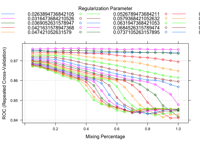
plot(model.glmnet.1)
set.seed(82)
model.glmnet.2 <- train(Survived ~ Pclass + Sex + Age + Embarked + Title + SibSp + Parch + TravelSize,
                        method = "glmnet",
                        tuneGrid = expand.grid(alpha = seq(0.05,1.0,.05), lambda = seq(0.0001, .01, length = 20)),
                        data = train.fit,
                        metric = "ROC",
                        trControl = fitControl) #No output, on purpose
plot(model.glmnet.2)
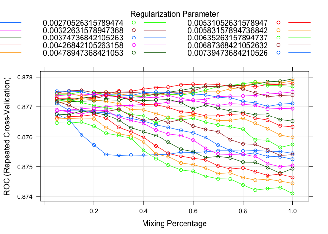
Like before, I setup two different glmnet models with just the Fare missing in one of them. I played around with the tuning a little to maximize the ROC value as well. Here I also plotted the models to see tuning parameters effect on the ROC value. The outcomes are relatively similar, but again we will use our validation sample later to determine which model is the best.
Boosted models
Next we can also test boosted methods. We used the gbm function earlier to estimate the missing Ages, and we can use it again here to estimate which passengers survived. It goes without saying that I will develop two models with the only difference being the Fare being included or not.
set.seed(82)
model.gbm.1 <- train(Survived ~ Pclass + Sex + Fare + Age + Embarked + Title + SibSp + Parch + TravelSize,
method = "gbm",
tuneGrid = expand.grid(interaction.depth = c(2, 3), n.trees = (1:30)*5, shrinkage = 0.1,
n.minobsinnode = 10),
data = train.fit,
metric = "ROC",
trControl = fitControl) #No output, on purpose
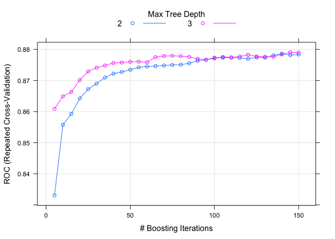
plot(model.gbm.1)
set.seed(82)
model.gbm.2 <- train(Survived ~ Pclass + Sex + Age + Embarked + Title + SibSp + Parch + TravelSize,
                        method = "gbm",
                        tuneGrid = expand.grid(interaction.depth = c(2, 3), n.trees = (5:40)*10, shrinkage = 0.1,
                        n.minobsinnode = 10),
                        data = train.fit,
                        metric = "ROC",
                        trControl = fitControl) #No output, on purpose
plot(model.gbm.2)
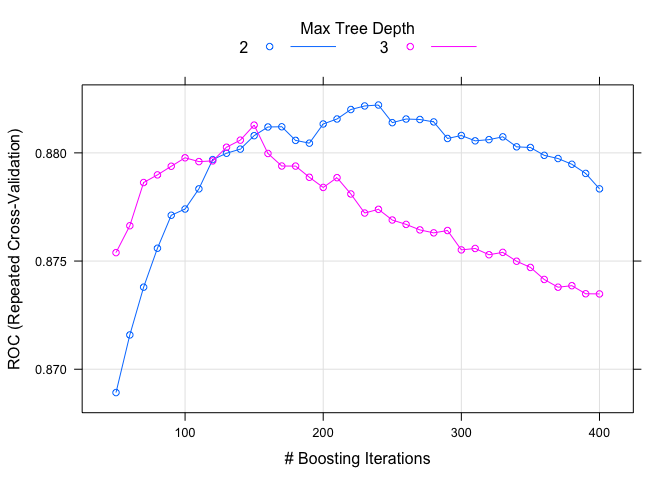
As before, I spent a little time tuning the models separately. There seems to be a small improvement in both gbm models compared to the previous ones. Another popular learning method is ‘adaptive boost’ using the ada package. The two boosted methods (gbm and ada) are quite similar. Let’s try it out.
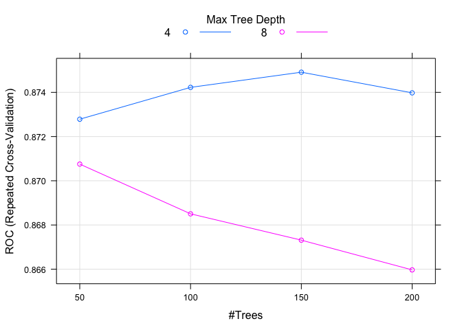
set.seed(82)
model.ada.1 <- train(Survived ~ Pclass + Sex + Fare + Age + Embarked + Title + SibSp + Parch + TravelSize,
                        method = "ada",
                        tuneGrid = expand.grid(.iter = seq(50, 200, 50), .maxdepth = c(4, 8), .nu = c(0.1)),
                        data = train.fit,
                        metric = "ROC",
                        trControl = fitControl) #No output, on purpose
plot(model.ada.1)
set.seed(82)
model.ada.2 <- train(Survived ~ Pclass + Sex + Age + Embarked + Title + SibSp + Parch + TravelSize,
                        method = "ada",
                        tuneGrid = expand.grid(.iter = c(50, 100), .maxdepth = c(4, 8), .nu = c(0.1, 1)),
                        data = train.fit,
                        metric = "ROC",
                        trControl = fitControl) #No output, on purpose
plot(model.ada.2)
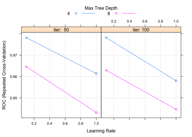
Not too surprisingly, the ada method performs roughly similar to gbm. Ultimately though, of course, the test.fit will be used to discern between all the models that we are creating. So we will see which one is the best then. Let’s move onto the last few models.
Other models
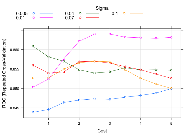
We will give support vector machine (SVM) a shot here. Using the kernlab package, we can fit the svmRadial method available. Here there are only two tunable parameters to play around with.
set.seed(82)
model.svm.1 <- train(Survived ~ Pclass + Sex + Fare + Age + Embarked + Title + SibSp + Parch + TravelSize,
                        method = "svmRadial",
                        preProcess = c("center", "scale"),
                        tuneGrid = expand.grid(C = seq(0.5, 5.0, 0.5), sigma = c(0.005, 0.01, 0.04, 0.07, 0.10)),
                        data = train.fit,
                        metric = "ROC",
                        trControl = fitControl) #No output, on purpose
plot(model.svm.1)
set.seed(82)
model.svm.2 <- train(Survived ~ Pclass + Sex + Age + Embarked + Title + SibSp + Parch + TravelSize,
                        method = "svmRadial",
                        preProcess = c("center", "scale"),
                        tuneGrid = expand.grid(C = seq(0.5, 5.0, 0.25), sigma = c(0.005, 0.01, 0.04, 0.07)),
                        data = train.fit,
                        metric = "ROC",
                        trControl = fitControl) #No output, on purpose
plot(model.svm.2)
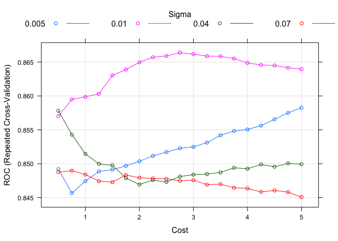
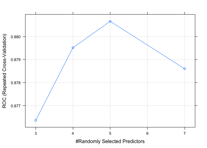
It seems the SVM models do not perform as well as either boosted models, at least in terms of the maximized ROC curve. This could be down to a number of reasons but again, we will have to wait to see how well they actually perform later. The last method I wanted to use is one of the most popular and easiest to use: random forest (RF). There is only one parameter to tune in train: number of (random) selectors to use in the fit. The general consensus is to use something close to the square root of the total independent variables. Since we have less than 10 variables, there is not much room for tuning, but let’s see what our last fit can do.
set.seed(82)
model.rf.1 <- train(Survived ~ Pclass + Sex + Fare + Age + Embarked + Title + SibSp + Parch + TravelSize,
                        method = "rf",
                        tuneGrid = data.frame(.mtry = c(3, 4, 5, 7)),
                        data = train.fit,
                        metric = "ROC",
                        trControl = fitControl) #No output, on purpose
plot(model.rf.1)
set.seed(82)
model.rf.2 <- train(Survived ~ Pclass + Sex + Age + Embarked + Title + SibSp + Parch + TravelSize,
                        method = "rf",
                        tuneGrid = data.frame(.mtry = c(3, 4, 5, 7)),
                        data = train.fit,
                        metric = "ROC",
                        trControl = fitControl) #No output, on purpose
plot(model.rf.2)
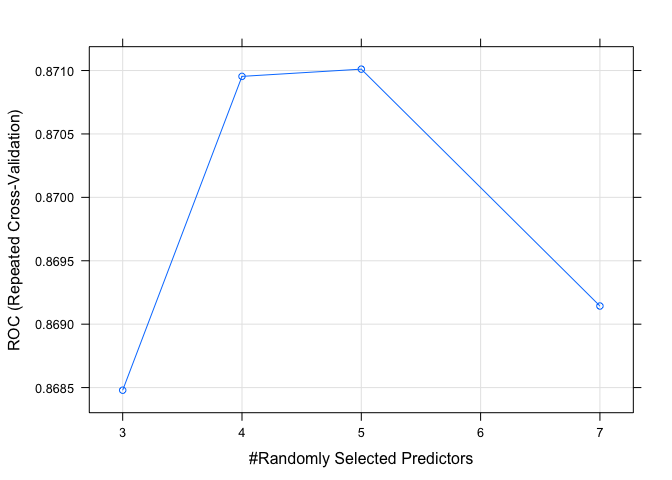
Both RF models perform as well as any of the other models tested. Since this is the last model I will test, we can now turn our attention at evaluating the models and choosing the best performer.
Model evaluation
With all our models trained and ready we can start comparing their performances. One way is the very handy confusionMatrix function which gives statistics on a model on a set of predicted data. This was a reason we kept some of the training data as a validation or test set. So let’s check out the output for one of our models.
pred.glm.1 <- predict(model.glm.1, test.fit)
confusionMatrix(pred.glm.1, test.fit$Survived)
## Confusion Matrix and Statistics
##
##           Reference
## Prediction Perished Survived
##   Perished       98       18
##   Survived       11       50
##
##                Accuracy : 0.8362
##                  95% CI : (0.7732, 0.8874)
##     No Information Rate : 0.6158
##     P-Value [Acc > NIR] : 1.38e-10
##
##                   Kappa : 0.6469
##  Mcnemar's Test P-Value : 0.2652
##
##             Sensitivity : 0.8991
##             Specificity : 0.7353
##          Pos Pred Value : 0.8448
##          Neg Pred Value : 0.8197
##              Prevalence : 0.6158
##          Detection Rate : 0.5537
##    Detection Prevalence : 0.6554
##       Balanced Accuracy : 0.8172
##
##        'Positive' Class : Perished
##
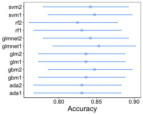
I will not show the output of the confusionMatrix for each model here, for brevity. Instead, I will plot the accuracy of each model (along with the 95% confidence intervals) so that we can compare them.
It is also useful to check the other statistics available to us. We can use the resamples method (again from the caret package) to resample the distributions and compare them. In fact, the output can easily be plotted with dotplot from lattice, though it does sort the data.
models <- list(glm1    = model.glm.1   , glm2    = model.glm.2,
               glmnet1 = model.glmnet.1, glmnet2 = model.glmnet.2,
               gbm1    = model.gbm.1   , gbm2    = model.gbm.2,
               ada1    = model.ada.1   , ada2    = model.ada.2,
               svm1    = model.svm.1   , svm2    = model.svm.2,
               rf1     = model.rf.1    , rf2     = model.rf.2)
model.val <- resamples(models)

dotplot(model.val)
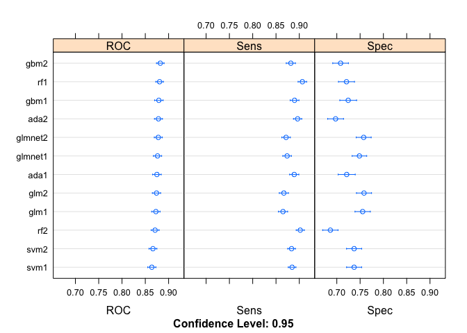
The Sensitivity is the probability to correctly identify a true positive while Specificity is the probability to correctly identify a true negative. Both values should be maximized where possible. Now that we have some statistics to be able to compare the models, we can try to determine the best one. Given what we have and the fact that I have to pick one, I am going to go with the first SVM model. By eye, it seems to have the best overall measures of the bunch.
Predictions
Having selected the SVM model, all we have left is to make a prediction and then submit to kaggle! Thankfully, this is also by far the easiest part.
the.prediction <- predict(model.svm.1, test.all)
the.solution <- data.frame(PassengerID = test.all$PassengerId, Survived = the.prediction)
the.solution$Survived <- revalue(the.solution$Survived, c("Survived" = 1, "Perished" = 0)) #Don't forget to revalue

write.csv(the.solution, file = "solution.csv", row.names = FALSE, quote = FALSE) #And write it out
After submitting this, we got a score of 0.78947: not too shabby. I am pretty happy with that score, as it does place in the top third of all entrants (currently).